Note: This post was originally published on AH’s Blog (WordPress) on April 25, 2017, and has been migrated here.

Key Terms

Vector Space Models (VSMs): Words represented as unique vectors, used as input to mathematical/statistical ML models.

Word Embedding: Fixed-size vector representations where semantically similar words have geometrically close vectors (small Euclidean distance). Used in Language Modeling, Machine Translation, and many NLP tasks.

Shallow Neural Networks: Neural networks with exactly 1 hidden (projection) layer, producing a new feature representation of the input.

One-Hot Encoding

The naive baseline. For a vocabulary V = {I, like, playing, football, basketball} (‖V‖ = 5):

I          = [1, 0, 0, 0, 0]
like       = [0, 1, 0, 0, 0]
playing    = [0, 0, 1, 0, 0]
football   = [0, 0, 0, 1, 0]
basketball = [0, 0, 0, 0, 1]

Pros: Simple, deterministic.

Cons: Vector size = vocabulary size (1M words → 1M-dim vectors). No semantic information — football and basketball are equally “distant” from each other as from “I”.

Use this when semantic relations don’t matter and vocabulary size is manageable.

Word2vec Philosophy

Word2vec represents a word using the words that surround it. Given:

“I like playing X”

Even without knowing what X is, the context (“like”, “playing”) tells us it’s something enjoyable and playable. This is exactly how humans infer meaning from context. Word2vec formalizes this: train a shallow neural network to predict context from a target word (or vice versa), and the learned weights become the word vectors.

Dataset

Corpus D:

"This battle will be my masterpiece"
"The unseen blade is the deadliest"

Vocabulary V = {this, battle, will, be, my, masterpiece, the, unseen, blade, is, deadliest}, ‖V‖ = 11

One-hot vectors (size 11) are assigned per word for use in the network.

Skip-gram Model

Task: Given a target word, predict its N surrounding context words.

Architecture: Input = one-hot vector of target word → 1 hidden (projection) layer → N Softmax output layers (one per context word to predict).

Example — target: “unseen”, context window = 3, embedding dimension = 3.

Input → Hidden (Wh, shape 11×3):

After feedforwarding “unseen”, hidden layer H = [0.8, 0.4, 0.5]. This is the initial embedding. Every row of Wh is the current embedding for each vocabulary word.

Hidden → Output:

Apply Softmax to each output vector, take the argmax index → predicted context words.

During training, errors from all N Softmax layers are averaged and backpropagated to update Wh. Repeat until max epochs or target loss is reached. The final input-to-hidden weight matrix is the word embedding.

Alternatively, the average of the Hidden-to-output weight matrices can serve as embeddings — but the input-to-hidden matrix is the standard choice.

Continuous Bag of Words (CBOW) Model

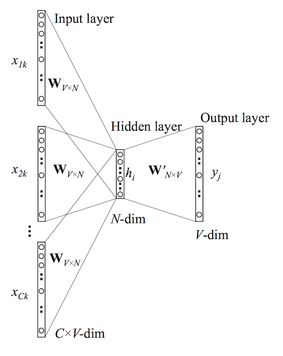
Task: Given N context words, predict the target word.

Architecture: N input one-hot vectors → 1 hidden layer (mean of input projections) → 1 Softmax output.

Example — target: “unseen”, context: “the”, “blade”, “is”.

Input → Hidden:

The hidden layer is the average of each context word’s projection:

H = [(0.8+0.2+0.2)/3, (0.9+0.8+0.3)/3, (0.1+0.9+0.7)/3] = [0.39, 0.66, 0.56]

Hidden → Output:

Apply Softmax → predicted word = “masterpiece” (in this initialization). Backpropagate error to update weights.

Conclusion

Word2vec is the bridge from symbolic NLP to semantic deep learning. Traditional rule-based systems fail to generalize across languages and cannot capture semantic similarity. One-hot encodings are equally blind to meaning. Word2vec vectors encode semantic proximity — enabling downstream models to reason about language.

Both Skip-gram and CBOW produce the same type of output (word embeddings) but differ in architecture: Skip-gram predicts context from a target; CBOW predicts a target from context. Skip-gram generally performs better on infrequent words; CBOW is faster to train on large corpora.

Part II covers negative sampling, hierarchical softmax, and practical training details.