
Another LSTM Tutorial
Note: This post was originally published on AH’s Blog (WordPress) on October 9, 2016, and has been migrated here.
Figures in this post are taken from Christopher Olah’s excellent Understanding LSTMs blog post.
Recurrent Neural Networks
Recurrent Neural Networks (RNNs) are designed for sequential data — data where order and dependency between elements matters. Traditional Multi-layer Perceptrons (MLPs) assume independence between inputs, which is inappropriate for text or audio.
RNNs contain self-loops that carry the previous hidden state forward, allowing the network to “remember” what it has seen.
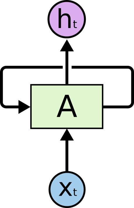
Unrolled over time, the RNN resembles a deep feedforward network where each step receives both the current input and the previous hidden state:

The Long-term Dependencies Problem
Standard RNNs have no mechanism to selectively forget irrelevant context. For a sentence like:
“I live in France, I like playing football with my friends and going to the school, I speak french”
Predicting “french” requires connecting to “I live in France” — but the two intermediate clauses introduce noise. Regular RNNs struggle to bridge these long-range dependencies, which is the main motivation behind LSTM.
What is LSTM?
Long Short-Term Memory (LSTM) is a variant of RNN that controls the memory process through gates within each unit. These gates regulate what information to retain, update, or forget, allowing the network to maintain relevant long-range context.
The analogy: when reading a novel, your brain selectively remembers important events (subject, previous action) while discarding irrelevant details. LSTMs simulate this selective memory.
LSTM Unit Structure

A standard LSTM unit contains:
- 2 inputs: previous cell state C_{t-1} and previous output h_{t-1}
- 4 layers: 3 sigmoid activations + 1 tanh activation
- 5 point operators: 3 multiplications, 1 addition, 1 tanh
- 2 outputs: current cell state C_t and current output h_t
The cell state is the memory backbone. It flows through the unit with minimal modification unless the gates decide to change it.
Detailed Processing: 3 Groups

Group 1.1 — Forget Gate

The forget gate layer (sigmoid) decides what to discard from the previous cell state. Output of 0 → forget everything; values closer to 1 → retain.

Group 1.2 — Applying Forget to Previous State

Element-wise multiply the forget gate output with C_{t-1}. A vector of zeros means we wipe all previous memory.

Group 2.1 — Input Gate and Candidate State

The input gate layer (sigmoid) decides which state values to update. A tanh layer generates the candidate new state values to potentially add.

Group 2.2 — Scaling New State

Multiply the candidate state by the input gate output to filter which new information actually gets written.

Combining Groups 1 + 2 → New Cell State

Add the filtered old state (Group 1) and filtered new information (Group 2) to get C_t.

Group 3 — Output Gate

A sigmoid layer decides which parts of the state to output. The state is passed through tanh (to keep values in [-1, 1]) and multiplied element-wise by the sigmoid output.

Conclusion
LSTMs have proven themselves across a wide range of tasks: Language Modeling, Sentiment Analysis, Speech Recognition, Text Summarization, and Question Answering. The gating mechanism is what makes them capable of learning which context to carry forward and which to discard.